Excel SUM Ranges – Tips to Avoid Devastating Errors

Once bitten, twice shy.  Spreadsheets have always been trying to bite us in the proverbial. Wolves in sheep's clothing.

Here's a real-life example...

Before Excel appeared I was responsible for building the annual budget for a company with some 30 departments, growing rapidly.  All was well. At the last moment, one department had two extra employees added, joining in month 3. The change was made in the spreadsheet.  The budget approved.  Backs slapped.

I was also responsible for the management reporting, and explaining budget variances.  Months 1 and 2 went OK. Then month 3 arrived.  A £5k adverse variance in one department.  Didn’t take long to find. The two new employees had joined as planned, but the budget didn’t include them. Two rows had been added to the department’s budget spreadsheet, but not picked up by the SUM formula. The costs had not been included.

As each month went by my embarrassment increased. Thankfully I didn’t have to refund the difference!

There are many other similar examples in businesses large and small. Lotus was sued for a similar problem in their 1-2-3 spreadsheet, but unsuccessfully. Using spreadsheet software accurately is down to the user.

So how do you stop such common and potentially disastrous errors?

• How to avoid making such errors? 
• How to check none have slipped through?

TIPS

Tip 1: Be aware of the dangers 

Firstly it pays to make sure everyone who uses Excel is aware of this risk and other spreadsheet risks.

Tip 2: Using blank rows at ends of ranges

The SUM range always adjusts if rows or columns are added within the SUM range. So:

• Insert an extra row above (or one column to the left of) the start of the numbers
• Insert an extra row (or column) after the range of numbers
• Use these extra rows/columns to at the start and end of the SUM ranges
• Reduce the height/width of these extra rows/columns (but ESSENTIAL not to hide them)
• Add a bottom border to the extra row (or to right of extra column)
• Only ever insert rows/columns between the pairs of blank rows/columns

There are two advantages over other tips below:

• The SUM can be placed anywhere in the spreadsheet, such as above or to the right, and the SUM will automatically adjust, even when start with 2 rows of numbers:

• If a row or column is added outside the SUM range, a warning is provided by the blank end-of-range rows/columns displaying oddly before adding the new figures:

Tip 3: Visualising the ranges

To provide a further check on a SUM range being  what you expect:

• Click on the cell containing the formula
• Then click anywhere on the formula appearing above the spreadsheet
• See the range highlighted (in blue)

Sadly this doesn’t work with the OFFSET function mentioned below, which is another reason not to use OFFSET.

But this method does also have the advantage of working with many other formulae to highlight the cells being used in the calculation. For example, only this week I copied a section that I had forgotten used a fixed cell (like $B$1) in formulae, when I had expected a new relative cell based on B1. I spotted the error before making the wrong financial decision!

Tip 4: Getting someone else to check it

Checking your own work is always tricky. The more edits are made that have to be re-checked, the more difficult this is.

Any spreadsheet that is of major importance should be checked by someone else. Including every ‘final’ version!



OTHER WAYS OF PREVENTING SUM RANGE ERRORS

There are some other techniques, which are covered here to show their pros and cons:

Tip 5: Automatic Excel feature

With Excel now by far the dominant spreadsheet, you would have hoped Microsoft would have done something to address the SUM range problem.  And they have.  But it is overly-complicated and works oddly:

• Under “Options” there is “Extend Data Range (or List) Formats and Formulas”, which should be ticked (usually by default). 
• Then set up a SUM range IMMEDIATELY BENEATH the bottom of a list of numbers (with no empty rows):
  
  
• Insert a row immediately above, and type in a number. The SUM range automatically expands to pick this up:
  
  
• Likewise if you insert multiple rows provided you enter numbers sequentially in each inserted row from the top. 

This automatic facility works similarly for a SUM across columns.  It even works if you insert the row/column, close the spreadsheet and reopen it.

But the SUM range does NOT automatically expand:

• If you don’t fill in the figures sequentially from the top, or leave a row blank (such as a row used for a sub-title)
  
• If the range started with only 2 rows
  
• The SUM is above, to the side or otherwise not directly below the range

The limitations apply similarly to SUM ranges across columns.

It is surprising this feature wasn’t implemented to adjust the SUM range as soon as the rows/columns are added, and to also cover 2 original rows.  But it wasn't. So this automatic feature is useful, but potentially fatally flawed.  Best not to rely on it.

Pros: Simple and works automatically most of the time
Cons: Easy to make mistakes when you think it would have worked

Tip 6: Modifying the SUM formula using OFFSET

You can manually achieve what Excel could have done, with a prompt for the syntax (from Excel 2010 onwards).

For a column of figures:

• Set up the formula in the format =SUM(C1: OFFSET(C5,-1,)) where C5 is the Total cell
• Usefully, the column letter automatically adjusts if the formula is copied across columns

For a row of figures across columns:

• Set up the formula in the very similar format =SUM(C1: OFFSET(G1,,-1)) where C5 is the Total cell

The formulae automatically change as soon as the row or column is inserted.

It also works if the total is at the top, or otherwise not immediately below the numbers, though you have to be extra careful with the range definition and subsequently adding rows/columns anywhere near the range.


Sadly “Offset” can slow down recalculations if used extensively in a spreadsheet.   So not perfect, but good if used carefully.

Pros: Reliable method
Cons: Not really any better than using blank rows in Tip 2 above, more difficult to set up, more difficult to check, and can slow down recalculation if used too much

Tip 7: Using 'Tables'


This tip can be useful when values in columns are being summed, i.e. the data is in rows. It doesn't work if cross-casting across columns.

If you insert a "Table" for the initial rows (even just two), you can put a normal SUM function below, above, or to the side of the column of numbers:

Add 2 rows above row 5, and all the totals will automatically adjust:

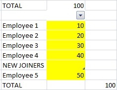
Add another two rows and put in the sub-heading "NEW JOINERS", and the totals still automatically adjusts:

If you don't initially put a SUM total immediately below the numbers, the other SUMs do NOT adjust unless the row headings are also in a Table column:

As you can see, the totals remain at 100 even after adding another 50. But there are two warnings that the totals are wrong:

•  The new rows are not shaded blue
• There is a little dark blue triangle in the bottom right corner  of the last cell (showing 40)

The problem can be avoided if the row headings are included in the Table:

If you don't want a column heading, set the cell colour to white, and the white writing doesn't show. You can also colour the number cells to a different colour, where you will still see the little dark blue triangle that marks the end of the SUM range:

You can also use Tables for multiple columns. But be careful! SUM ranges that are copied right do not automatically adjust for the columns, as you might expect. You have to set each column total separately:

Ranges have pros but some significant cons. Can be useful if used with care.

Pros: Useful if using Tables as a simple database
Cons: Unrelieable and less useful in financial modelling, as formulae do not copy right properly, and can cause errors if not used carefully. Colouring may not be desirable.

CHECKING SUM RANGES

Assuming you don’t have any Excel auditing software that can assist, there is another way of checking SUM ranges:


Tip 8: Re-calculating SUM

Instead of getting Excel to show the range, highlight the relevant range manually and Excel will display the SUM in the bottom bar. This can be easily compared to the SUM being displayed in the spreadsheet itself. This DOES work with the OFFSET function.

Pros: Quick and simple, and works if use OFFSET
Cons: Only works for SUM (and COUNT and AVERAGE) formulae

IN CONCLUSION

Spreadsheets are powerful but dangerous things. It is easy to make a material error in something as simple and important as adding a range of figures.

1. The first step is to realise there is a danger. 
2. Reduce the risk of error by using Tip 2 by adding blank rows/columns at ends of SUM ranges
3. Review formulae as in tip 3 
4. Use the other tips and techniques when circumstances are appropriate
5. Get someone else to check the spreadsheet model

Microsoft Responds. Or Have They?

News reaches us today that Microsoft have confirmed that all the limitations of Excel for forecasting listed in our recent blog article will be addressed in the next release of Excel. 

Or have they?